Using Compose with Featuretools

In this guide, we will generate labels and features on a mock dataset of transactions using Compose and Featuretools. Then create a machine learning model for predicting one hour in advance whether customers will spend over $1200 within the next hour of transactions.

%matplotlib inline
import composeml as cp
import featuretools as ft
import pandas as pd
from sklearn.model_selection import train_test_split
from sklearn.ensemble import RandomForestClassifier
from sklearn.metrics import classification_report

Load Data

To get an idea on how the transactions looks, we preview the data frame.

transactions = ft.demo.load_mock_customer(
    return_single_table=True,
    random_seed=0,
)

transactions[transactions.columns[:7]].head()

	transaction_id	session_id	transaction_time	product_id	amount	customer_id	device
0	298	1	2014-01-01 00:00:00	5	127.64	2	desktop
1	10	1	2014-01-01 00:09:45	5	57.39	2	desktop
2	495	1	2014-01-01 00:14:05	5	69.45	2	desktop
3	460	10	2014-01-01 02:33:50	5	123.19	2	tablet
4	302	10	2014-01-01 02:37:05	5	64.47	2	tablet

Generate Labels

Now with the transactions loaded, we are ready to generate labels for our prediction problem.

Create Labeling Function

First, we define the function that will return the total purchase amount given a hour of transactions.

def total_spent(df):
    total = df["amount"].sum()
    return total

Construct Label Maker

With our labeling function, we create the LabelMaker for the transactions. The target_entity is set to customer_id so that the labels are generated for each customer. The window_size is set to one hour to process one hour of transactions for a given customer.

label_maker = cp.LabelMaker(
    target_entity='customer_id',
    time_index='transaction_time',
    labeling_function=total_spent,
    window_size='1h',
)

Create Labels

Next, we automatically search and extract the labels by using LabelMaker.search().

See also

For more details on how the label maker works, see Main Concepts.

labels = label_maker.search(
    transactions.sort_values('transaction_time'),
    num_examples_per_instance=-1,
    gap=1,
)

labels.head()

Elapsed: 00:00 | Remaining: 00:00 | Progress: 100%|██████████| customer_id: 5/5

	customer_id	time	total_spent
id
0	1	2014-01-01 00:44:25	2880.53
1	1	2014-01-01 00:45:30	2859.18
2	1	2014-01-01 00:46:35	2751.07
3	1	2014-01-01 00:47:40	2638.54
4	1	2014-01-01 00:48:45	2632.25

Transform Labels

With the generated LabelTimes, we will apply specific transforms for our prediction problem.

Apply Threshold on Labels

We apply LabelTimes.threshold() to make the labels binary for total amounts exceeding $1200.

labels = labels.threshold(1200)

labels.head()

	customer_id	time	total_spent
id
0	1	2014-01-01 00:44:25	True
1	1	2014-01-01 00:45:30	True
2	1	2014-01-01 00:46:35	True
3	1	2014-01-01 00:47:40	True
4	1	2014-01-01 00:48:45	True

Lead Label Times

We also use LabelTimes.apply_lead() to shift the label times 1 hour earlier for predicting in advance.

labels = labels.apply_lead('1h')

labels.head()

	customer_id	time	total_spent
id
0	1	2013-12-31 23:44:25	True
1	1	2013-12-31 23:45:30	True
2	1	2013-12-31 23:46:35	True
3	1	2013-12-31 23:47:40	True
4	1	2013-12-31 23:48:45	True

Describe Labels

After transforming the labels, we could use LabelTimes.describe() to print out the distribution with the settings and transforms that were used to make the labels. This is useful as a reference for understanding how the labels were generated from raw data. Also, the label distribution is helpful for determining if we have imbalanced labels.

labels.describe()

Label Distribution
------------------
False     248
True      252
Total:    500


Settings
--------
gap                                    1
label_type                      discrete
labeling_function            total_spent
minimum_data                        None
num_examples_per_instance             -1
target_entity                customer_id
window_size                       <Hour>


Transforms
----------
1. threshold
  - value:    1200

2. apply_lead
  - value:    1h

Generate Features

Now with the generated labels, we are ready to generate features for our prediction problem.

Create Entity Set

Let’s construct an EntitySet and load the transactions as an entity by using EntitySet.entity_from_dataframe(). Then extract additional entities by using EntitySet.normalize_entity().

See also

For more details on working with entity sets, see loading_data/using_entitysets .

es = ft.EntitySet('transactions')

es.entity_from_dataframe(
    'transactions',
    transactions,
    index='transaction_id',
    time_index='transaction_time',
)

es.normalize_entity(
    base_entity_id='transactions',
    new_entity_id='sessions',
    index='session_id',
    make_time_index='session_start',
    additional_variables=[
        'device',
        'customer_id',
        'zip_code',
        'session_start',
        'join_date',
        'date_of_birth',
    ],
)

es.normalize_entity(
    base_entity_id='sessions',
    new_entity_id='customers',
    index='customer_id',
    make_time_index='join_date',
    additional_variables=[
        'zip_code',
        'join_date',
        'date_of_birth',
    ],
)

es.normalize_entity(
    base_entity_id='transactions',
    new_entity_id='products',
    index='product_id',
    additional_variables=['brand'],
    make_time_index=False,
)

es.add_last_time_indexes()

Describe Entity Set

To get information on how the entity set is structured, we could print the entity set and use EntitySet.plot() to create a diagram.

print(es, end='\n\n')

es.plot()

Entityset: transactions
  Entities:
    transactions [Rows: 500, Columns: 5]
    sessions [Rows: 35, Columns: 4]
    customers [Rows: 5, Columns: 4]
    products [Rows: 5, Columns: 2]
  Relationships:
    transactions.session_id -> sessions.session_id
    sessions.customer_id -> customers.customer_id
    transactions.product_id -> products.product_id

Create Feature Matrix

Next, we generate features that correspond to the labels created previously by using dfs(). The target_entity is set to customers so that features are only calculated for customers. The cutoff_time is set to the labels so that features are calculated only using data up to and including the label cutoff times. Notice that the output of Compose integrates easily with Featuretools.

See also

For more details on calculating features using cutoff times, see automated_feature_engineering/handling_time.

feature_matrix, features_defs = ft.dfs(
    entityset=es,
    target_entity='customers',
    cutoff_time=labels,
    cutoff_time_in_index=True,
    verbose=True,
)

Built 77 features
Elapsed: 00:51 | Progress: 100%|██████████

Describe Features

To get an idea on how the generated features look, we preview the feature definitions.

features_defs[:20]

[<Feature: zip_code>,
 <Feature: COUNT(sessions)>,
 <Feature: NUM_UNIQUE(sessions.device)>,
 <Feature: MODE(sessions.device)>,
 <Feature: SUM(transactions.amount)>,
 <Feature: STD(transactions.amount)>,
 <Feature: MAX(transactions.amount)>,
 <Feature: SKEW(transactions.amount)>,
 <Feature: MIN(transactions.amount)>,
 <Feature: MEAN(transactions.amount)>,
 <Feature: COUNT(transactions)>,
 <Feature: NUM_UNIQUE(transactions.product_id)>,
 <Feature: MODE(transactions.product_id)>,
 <Feature: DAY(date_of_birth)>,
 <Feature: DAY(join_date)>,
 <Feature: YEAR(date_of_birth)>,
 <Feature: YEAR(join_date)>,
 <Feature: MONTH(date_of_birth)>,
 <Feature: MONTH(join_date)>,
 <Feature: WEEKDAY(date_of_birth)>]

Machine Learning

Now with the generated labels and features, we are ready to create a machine learning model for our prediction problem.

Preprocess Features

In the feature matrix, let’s extract the labels and fill any missing values with zeros. Then, one-hot encode all categorical features by using encode_features().

y = feature_matrix.pop('total_spent')
x = feature_matrix.fillna(0)
x, features_enc = ft.encode_features(x, features_defs)

Split Labels and Features

After preprocessing, we split the features and corresponding labels each into training and testing sets.

x_train, x_test, y_train, y_test = train_test_split(
    x,
    y,
    train_size=.8,
    test_size=.2,
    random_state=0,
)

Train Model

Next, we train a random forest classifer on the training set.

clf = RandomForestClassifier(n_estimators=10, random_state=0)

clf.fit(x_train, y_train)

RandomForestClassifier(bootstrap=True, class_weight=None, criterion='gini',
                       max_depth=None, max_features='auto', max_leaf_nodes=None,
                       min_impurity_decrease=0.0, min_impurity_split=None,
                       min_samples_leaf=1, min_samples_split=2,
                       min_weight_fraction_leaf=0.0, n_estimators=10,
                       n_jobs=None, oob_score=False, random_state=0, verbose=0,
                       warm_start=False)

Test Model

Lastly, we test the model performance by evaluating predictions on the testing set.

y_hat = clf.predict(x_test)

print(classification_report(y_test, y_hat))

              precision    recall  f1-score   support

       False       0.79      0.90      0.84        49
        True       0.89      0.76      0.82        51

    accuracy                           0.83       100
   macro avg       0.84      0.83      0.83       100
weighted avg       0.84      0.83      0.83       100

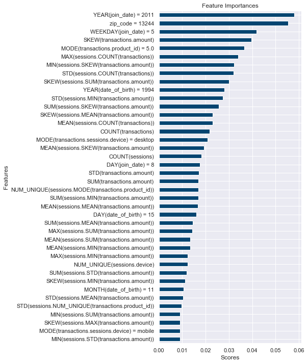
Feature Importances

This plot is based on scores obtained by the model to illustrate which features are considered important for predictions.

feature_importances = zip(x_train.columns, clf.feature_importances_)
feature_importances = pd.Series(dict(feature_importances))
feature_importances = feature_importances.rename_axis('Features')
feature_importances = feature_importances.sort_values()

top_features = feature_importances.tail(40)
plot = top_features.plot(kind='barh', figsize=(5, 12), color='#054571')
plot.set_title('Feature Importances')
plot.set_xlabel('Scores');