Getting Started

In this example, we will generate labels on a mock dataset of transactions. For each customer, we want to label whether the total purchase amount over the next hour of transactions will exceed $300. Additionally, we want to predict one hour in advance.

import composeml as cp

Load Data

With the package installed, we load in the data. To get an idea on how the transactions looks, we preview the data frame.

df = cp.demos.load_transactions()

df[df.columns[:7]].head()

	transaction_id	session_id	transaction_time	product_id	amount	customer_id	device
0	298	1	2014-01-01 00:00:00	5	127.64	2	desktop
1	10	1	2014-01-01 00:09:45	5	57.39	2	desktop
2	495	1	2014-01-01 00:14:05	5	69.45	2	desktop
3	460	10	2014-01-01 02:33:50	5	123.19	2	tablet
4	302	10	2014-01-01 02:37:05	5	64.47	2	tablet

Create Labeling Function

To get started, we define the labeling function that will return the total purchase amount given a hour of transactions.

def total_spent(df):
    total = df['amount'].sum()
    return total

Construct Label Maker

With the labeling function, we create the LabelMaker for our prediction problem. To process one hour of transactions for each customer, we set the target_entity to the customer ID and the window_size to one hour.

label_maker = cp.LabelMaker(
    target_entity="customer_id",
    time_index="transaction_time",
    labeling_function=total_spent,
    window_size="1h",
)

Generate Labels

Next, we automatically search and extract the labels by using LabelMaker.search().

labels = label_maker.search(
    df.sort_values('transaction_time'),
    num_examples_per_instance=-1,
    gap=1,
    verbose=True,
)

labels.head()

Elapsed: 00:00 | Remaining: 00:00 | Progress: 100%|██████████| customer_id: 5/5

	customer_id	time	total_spent
0	1	2014-01-01 00:45:30	914.73
1	1	2014-01-01 00:46:35	806.62
2	1	2014-01-01 00:47:40	694.09
3	1	2014-01-01 00:52:00	687.80
4	1	2014-01-01 00:53:05	656.43

Transform Labels

With the generated LabelTimes, we will apply specific transforms for our prediction problem.

Apply Threshold on Labels

To make the labels binary, LabelTimes.threshold() is applied for amounts exceeding $300.

labels = labels.threshold(300)

labels.head()

	customer_id	time	total_spent
0	1	2014-01-01 00:45:30	True
1	1	2014-01-01 00:46:35	True
2	1	2014-01-01 00:47:40	True
3	1	2014-01-01 00:52:00	True
4	1	2014-01-01 00:53:05	True

Lead Label Times

Additionally, the label times are shifted one hour earlier for predicting in advance by using LabelTimes.apply_lead().

labels = labels.apply_lead('1h')

labels.head()

	customer_id	time	total_spent
0	1	2013-12-31 23:45:30	True
1	1	2013-12-31 23:46:35	True
2	1	2013-12-31 23:47:40	True
3	1	2013-12-31 23:52:00	True
4	1	2013-12-31 23:53:05	True

Describe Labels

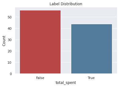
After transforming the labels, we can use LabelTimes.describe() to print out the distribution with the settings and transforms that were used to make these labels. This is useful as a reference for understanding how the labels were generated from raw data. Also, the label distribution is helpful for determining if we have imbalanced labels.

labels.describe()

Label Distribution
------------------
False      56
True       44
Total:    100


Settings
--------
gap                                    1
minimum_data                        None
num_examples_per_instance             -1
target_column                total_spent
target_entity                customer_id
target_type                     discrete
window_size                       <Hour>


Transforms
----------
1. threshold
  - value:    300

2. apply_lead
  - value:    1h

Plot Labels

Also, there are plots available for insight to the labels.

Distribution

This plot shows the label distribution.

%matplotlib inline
labels.plot.distribution();

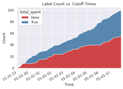
Count by Time

This plot shows the label distribution across cutoff times.

%matplotlib inline
labels.plot.count_by_time();