Predict Remaining Useful Life

In this example, we will generate labels using Compose on data provided by NASA simulating turbofan engine degradation. Then, the labels are used to generate features and train a machine learning model to predict the Remaining Useful Life (RUL) of an engine.

%matplotlib inline
import composeml as cp
import featuretools as ft
import pandas as pd
import data

from sklearn.model_selection import train_test_split
from sklearn.ensemble import RandomForestClassifier
from sklearn.metrics import classification_report

Load Data

In this dataset, we have 249 engines (engine_no) which are monitored over time (time_in_cycles). Each engine had operational_settings and sensor_measurements recorded for each cycle. The Remaining Useful Life (RUL) is the amount of cycles an engine has left before it needs maintenance. What makes this dataset special is that the engines run all the way until failure, giving us precise RUL information for every engine at every point in time.

You can download the data directly from NASA here. After downloading the data, you can set the file parameter as an absolute path to train_FD004.txt. With the file in place, we preview the data to get an idea on how to observations look.

df = data.load('data/train_FD004.txt')
df[df.columns[:7]].head()

	engine_no	time_in_cycles	operational_setting_1	operational_setting_2	operational_setting_3	sensor_measurement_1	sensor_measurement_2
0	1	1	42.0049	0.8400	100.0	445.00	549.68
1	1	2	20.0020	0.7002	100.0	491.19	606.07
2	1	3	42.0038	0.8409	100.0	445.00	548.95
3	1	4	42.0000	0.8400	100.0	445.00	548.70
4	1	5	25.0063	0.6207	60.0	462.54	536.10

Generate Labels

Now with the observations loaded, we are ready to generate labels for our prediction problem.

Define Labeling Function

To get started, we define the labeling function that will return the RUL given the remaining observations of an engine.

def remaining_useful_life(df):
    return len(df) - 1

Create Label Maker

With the labeling function, we create the label maker for our prediction problem. To process the RUL for each engine, we set the target_entity to the engine number. By default, the window_size is set to the total observation size to contain the remaining observations for each engine.

lm = cp.LabelMaker(
    target_entity='engine_no',
    time_index='time',
    labeling_function=remaining_useful_life,
)

Search Labels

Let’s imagine we want to make predictions on turbines that are up and running. Turbines in general don’t fail before 120 cycles, so we will only make labels for engines that reach at least 100 cycles. To do this, the minimum_data parameter is set to 100. Using Compose, we can easily tweak this parameter as the requirements of our model changes. Additionally, we set gap to one to create labels on every cycle and limit the search to 10 examples for each engine.

See also

For more details on how the label maker works, see Main Concepts.

lt = lm.search(
    df.sort_values('time'),
    num_examples_per_instance=10,
    minimum_data=100,
    gap=1,
    verbose=True,
)

lt.head()

Elapsed: 00:01 | Remaining: 00:00 | Progress: 100%|██████████| engine_no: 2490/2490

	engine_no	time	remaining_useful_life
id
0	1	2000-01-01 16:40:00	220
1	1	2000-01-01 16:50:00	219
2	1	2000-01-01 17:00:00	218
3	1	2000-01-01 17:10:00	217
4	1	2000-01-01 17:20:00	216

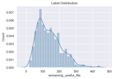
Continuous Labels

The labeling function we defined returns continuous labels which can be used to train a regression model for our predictin problem. Alternatively, there are label transforms available to further process these labels into discrete values. In which case, can be used to train a classification model.

Describe Labels

Let’s print out the settings and transforms that were used to make the continuous labels. This is useful as a reference for understanding how the labels were generated from raw data.

lt.describe()

Settings
--------
gap                                              1
label_type                              continuous
labeling_function            remaining_useful_life
minimum_data                                   100
num_examples_per_instance                       10
target_entity                            engine_no
window_size                                  61249


Transforms
----------
No transforms applied

Let’s plot the labels to get additional insight of the RUL.

Label Distribution

This plot shows the continuous label distribution.

lt.plot.distribution();

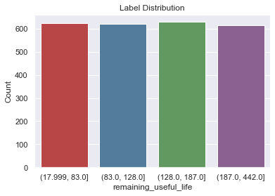
Discrete Labels

Let’s further process the labels into discrete values. We divide the RUL into quartile bins to predict which range an engine’s RUL will fall in.

lt = lt.bin(4, quantiles=True)

Describe Labels

Next, let’s print out the settings and transforms that were used to make the discrete labels. This time we can see the label distribution which is useful for determining if we have imbalanced labels. Also, we can see that the label type changed from continuous to discrete and the binning transform used in the previous step is included below.

lt.describe()

Label Distribution
------------------
(128.0, 187.0]     629
(17.999, 83.0]     625
(187.0, 442.0]     614
(83.0, 128.0]      622
Total:            2490


Settings
--------
gap                                              1
label_type                                discrete
labeling_function            remaining_useful_life
minimum_data                                   100
num_examples_per_instance                       10
target_entity                            engine_no
window_size                                  61249


Transforms
----------
1. bin
  - bins:            4
  - labels:       None
  - quantiles:    True
  - right:        True

Let’s plot the labels to get additional insight of the RUL.

Label Distribution

This plot shows the discrete label distribution.

lt.plot.distribution();

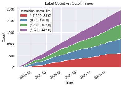
Count by Time

This plot shows the label count accumulated across cutoff times.

lt.plot.count_by_time();

Generate Features

Now, we are ready to generate features for our prediction problem.

Create Entity Set

To get started, let’s create an EntitySet for the observations.

See also

For more details on working with entity sets, see loading_data/using_entitysets.

es = ft.EntitySet('observations')

es.entity_from_dataframe(
    dataframe=df,
    entity_id='recordings',
    index='id',
    time_index='time',
    make_index=True,
)

es.normalize_entity(
    base_entity_id='recordings',
    new_entity_id='engines',
    index='engine_no',
)

es.normalize_entity(
    base_entity_id='recordings',
    new_entity_id='cycles',
    index='time_in_cycles',
)

Entityset: observations
  Entities:
    recordings [Rows: 61249, Columns: 28]
    engines [Rows: 249, Columns: 2]
    cycles [Rows: 543, Columns: 2]
  Relationships:
    recordings.engine_no -> engines.engine_no
    recordings.time_in_cycles -> cycles.time_in_cycles

Describe Entity Set

To get an idea on how the entity set is structured, we can plot a diagram.

es.plot()

Create Feature Matrix

To simplify the calculation for the feature matrix, we only use 20 percent of the labels.

lt = lt.sample(frac=.2, random_state=0)

Let’s generate features that correspond to the labels. To do this, we set the target_entity to engines and the cutoff_time to our labels so that the features are calculated for each engine only using data up to and including the cutoff time of each label. Notice that the output of Compose integrates easily with Featuretools.

See also

For more details on calculating features using cutoff times, see automated_feature_engineering/handling_time.

fm, fd = ft.dfs(
    entityset=es,
    target_entity='engines',
    agg_primitives=['last', 'max', 'min'],
    trans_primitives=[],
    cutoff_time=lt,
    cutoff_time_in_index=True,
    max_depth=3,
    verbose=True,
)

fm.head()

Built 292 features
Elapsed: 03:05 | Progress: 100%|██████████

		LAST(recordings.sensor_measurement_2)	LAST(recordings.sensor_measurement_21)	LAST(recordings.sensor_measurement_1)	LAST(recordings.sensor_measurement_4)	LAST(recordings.sensor_measurement_5)	LAST(recordings.sensor_measurement_11)	LAST(recordings.sensor_measurement_7)	LAST(recordings.sensor_measurement_9)	LAST(recordings.sensor_measurement_19)	LAST(recordings.sensor_measurement_18)	...	MIN(recordings.cycles.LAST(recordings.sensor_measurement_11))	MIN(recordings.cycles.LAST(recordings.sensor_measurement_3))	MIN(recordings.cycles.MIN(recordings.sensor_measurement_16))	MIN(recordings.cycles.MAX(recordings.operational_setting_1))	MIN(recordings.cycles.LAST(recordings.sensor_measurement_18))	MIN(recordings.cycles.MIN(recordings.sensor_measurement_17))	MIN(recordings.cycles.MAX(recordings.operational_setting_3))	MIN(recordings.cycles.MIN(recordings.sensor_measurement_10))	MIN(recordings.cycles.MAX(recordings.sensor_measurement_18))	remaining_useful_life
engine_no	time
233	2001-02-02 07:30:00	643.08	23.3473	518.67	1399.84	14.62	47.49	554.09	9068.13	100.00	2388	...	36.49	1250.55	0.02	42.0070	1915	302	100.0	0.93	2388	(128.0, 187.0]
146	2000-09-04 07:50:00	554.79	8.8768	449.44	1118.14	5.48	41.61	195.73	8346.50	100.00	2223	...	36.45	1254.83	0.02	42.0067	1915	302	100.0	0.93	2388	(187.0, 442.0]
105	2000-06-26 11:10:00	549.28	6.3080	445.00	1127.19	3.91	42.03	139.18	8332.78	100.00	2212	...	36.36	1251.50	0.02	42.0067	1915	302	100.0	0.93	2388	(17.999, 83.0]
240	2001-02-13 23:20:00	642.73	23.2631	518.67	1411.59	14.62	47.50	552.91	9048.65	100.00	2388	...	36.39	1251.07	0.02	42.0070	1915	302	100.0	0.93	2388	(17.999, 83.0]
229	2001-01-26 09:00:00	536.44	8.5711	462.54	1047.57	7.05	36.54	174.64	8008.89	84.93	1915	...	36.43	1249.84	0.02	42.0070	1915	302	100.0	0.93	2388	(128.0, 187.0]

5 rows × 293 columns

Machine Learning

Now, we are ready to create a machine learning model for our prediction problem.

Preprocess Features

Let’s extract the labels from the feature matrix and fill any missing values with zeros. Additionally, the categorical features are one-hot encoded.

y = fm.pop('remaining_useful_life')
y = y.astype('str')

x = fm.fillna(0)
x, fe = ft.encode_features(x, fd)

Split Labels and Features

Then, we split the labels and features each into training and testing sets.

x_train, x_test, y_train, y_test = train_test_split(
    x,
    y,
    train_size=.8,
    test_size=.2,
    random_state=0,
)

Train Model

Next, we train a random forest classifer on the training set.

clf = RandomForestClassifier(n_estimators=10, random_state=0)
clf.fit(x_train, y_train)

RandomForestClassifier(bootstrap=True, class_weight=None, criterion='gini',
                       max_depth=None, max_features='auto', max_leaf_nodes=None,
                       min_impurity_decrease=0.0, min_impurity_split=None,
                       min_samples_leaf=1, min_samples_split=2,
                       min_weight_fraction_leaf=0.0, n_estimators=10,
                       n_jobs=None, oob_score=False, random_state=0, verbose=0,
                       warm_start=False)

Test Model

Lastly, we test the model performance by evaluating predictions on the testing set.

y_hat = clf.predict(x_test)
print(classification_report(y_test, y_hat))

                precision    recall  f1-score   support

(128.0, 187.0]       0.65      0.79      0.71        28
(17.999, 83.0]       0.64      0.73      0.68        22
(187.0, 442.0]       0.81      0.84      0.82        25
 (83.0, 128.0]       0.67      0.40      0.50        25

      accuracy                           0.69       100
     macro avg       0.69      0.69      0.68       100
  weighted avg       0.69      0.69      0.68       100

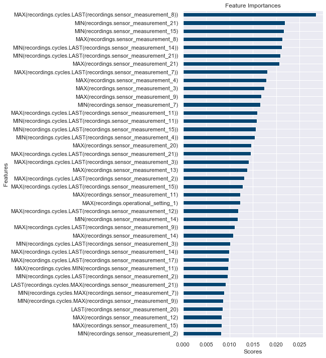
Feature Importances

This plot is based on scores from the model to show which features are important for predictions.

feature_importances = zip(x_train.columns, clf.feature_importances_)
feature_importances = pd.Series(dict(feature_importances))
feature_importances = feature_importances.rename_axis('Features')
feature_importances = feature_importances.sort_values()

top_features = feature_importances.tail(40)
plot = top_features.plot(kind='barh', figsize=(5, 12), color='#054571')
plot.set_title('Feature Importances')
plot.set_xlabel('Scores');