Predict Next Purchase

In this example, we build a machine learning application to predict whether customers will purchase a product within the next shopping period. This application is structured into three important steps:

• Prediction Engineering

• Feature Engineering

• Machine Learning

In the first step, we generate new labels from the data by using Compose. In the second step, we generate features for the labels by using Featuretools. In the third step, we search for the best machine learning pipeline by using EvalML. After working through these steps, you will learn how to build machine learning applications for real-world problems like predicting consumer spending. Let’s get started.

from demo.next_purchase import load_sample
from matplotlib.pyplot import subplots
import composeml as cp
import featuretools as ft
import evalml

We will use this historical data of online grocery orders provided by Instacart.

df = load_sample()

df.head()

	order_id	product_id	add_to_cart_order	reordered	product_name	aisle_id	department_id	department	user_id	order_time
id
0	120	33120	13	0	Organic Egg Whites	86	16	dairy eggs	23750	2015-01-11 08:00:00
1	120	31323	7	0	Light Wisconsin String Cheese	21	16	dairy eggs	23750	2015-01-11 08:00:00
2	120	1503	8	0	Low Fat Cottage Cheese	108	16	dairy eggs	23750	2015-01-11 08:00:00
3	120	28156	11	0	Total 0% Nonfat Plain Greek Yogurt	120	16	dairy eggs	23750	2015-01-11 08:00:00
4	120	41273	4	0	Broccoli Florets	123	4	produce	23750	2015-01-11 08:00:00

Prediction Engineering

Will customers purchase a product within the next shopping period?

In this prediction problem, we have two parameters:

• The product that a customer can purchase.

• The length of the shopping period.

We can change these parameters to create different prediction problems. For example, will a customer purchase a banana within the next 5 days or an avocado within the next three weeks? These variations can be done by simply tweaking the parameters. This helps us explore different scenarios which is crucial for making better decisions.

Defining the Labeling Process

Let’s start by defining a labeling function that checks if a customer bought a given product. We will make the product a parameter of the function.

def bought_product(ds, product_name):
    return ds.product_name.str.contains(product_name).any()

Representing the Prediction Problem

Then, let’s represent the prediction problem by creating a label maker with the following parameters:

• target_entity as the columns for the customer ID, since we want to process orders for each customer.

• labeling_function as the function we defined previously.

• time_index as the column for the order time. The shoppings periods are based on this time index.

• window_size as the length of a shopping period. We can easily change this parameter to create variations of the prediction problem.

lm = cp.LabelMaker(
    target_entity='user_id',
    time_index='order_time',
    labeling_function=bought_product,
    window_size='3d',
)

Finding the Training Examples

Now, let’s run a search to get the training examples by using the following parameters:

• The grocery orders sorted by the order time.

• num_examples_per_instance to find the number of training examples per customer. In this case, the search will return all existing examples.

• product_name as the product to check for purchases. This parameter gets passed directly to the our labeling function.

• minimum_data as the amount of data that will be used to make features for the first training example.

lt = lm.search(
    df.sort_values('order_time'),
    num_examples_per_instance=-1,
    product_name='Banana',
    minimum_data='3d',
    verbose=False,
)

lt.head()

	user_id	time	bought_product
0	2555	2015-01-22 09:00:00	False
1	3283	2015-01-08 13:00:00	True
2	5360	2015-01-21 11:00:00	False
3	5669	2015-01-09 08:00:00	False
4	5669	2015-01-12 08:00:00	True

The output from the search is a label times table with three columns:

• The customer ID associated to the orders.

• The start time of the shopping period. This is also the cutoff time for building features. Only data that existed beforehand is valid to use for predictions.

• Whether or not the product was purchased. This is calculated by our labeling function.

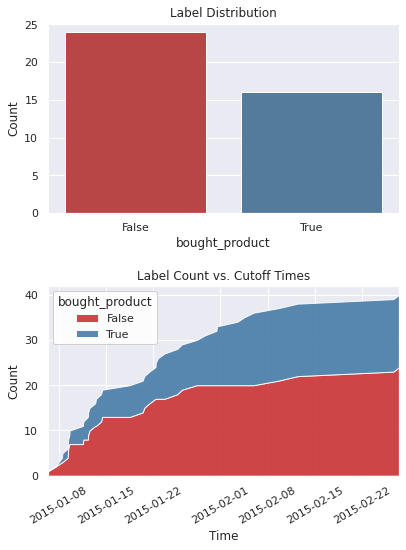
As a helpul reference, we can print out the search settings that were used to generate these labels. The description also shows us the label distribution which we can check for imbalanced labels.

lt.describe()

Label Distribution
------------------
False     24
True      16
Total:    40


Settings
--------
gap                                    None
minimum_data                             3d
num_examples_per_instance                -1
target_column                bought_product
target_entity                       user_id
target_type                        discrete
window_size                              3d


Transforms
----------
No transforms applied

We can also get a better look at the labels by plotting the distribution and cumulative count across time.

%matplotlib inline
fig, ax = subplots(nrows=2, ncols=1, figsize=(6, 8))
lt.plot.distribution(ax=ax[0])
lt.plot.count_by_time(ax=ax[1])
fig.tight_layout(pad=2)

Feature Engineering

In the previous step, we generated the labels. The next step is to generate the features.

Representing the Data

We will represent the online grocery orders using an entity set. This way, we can generate features based on the relational structure of the dataset. We currently have a single table of orders where one customer can many orders. This one-to-many relationship can be represented by normalizing an entity for customers. The same can be done for departments, aisles, and products. Let’s structure the entity set.

es = ft.EntitySet('instacart')

es.entity_from_dataframe(
    dataframe=df.reset_index(),
    entity_id='order_products',
    time_index='order_time',
    index='id',
)

es.normalize_entity(
    base_entity_id='order_products',
    new_entity_id='orders',
    index='order_id',
    additional_variables=['user_id'],
    make_time_index=False,
)

es.normalize_entity(
    base_entity_id='orders',
    new_entity_id='customers',
    index='user_id',
    make_time_index=False,
)

es.normalize_entity(
    base_entity_id='order_products',
    new_entity_id='products',
    index='product_id',
    additional_variables=['aisle_id', 'department_id'],
    make_time_index=False,
)

es.normalize_entity(
    base_entity_id='products',
    new_entity_id='aisles',
    index='aisle_id',
    additional_variables=['department_id'],
    make_time_index=False,
)

es.normalize_entity(
    base_entity_id='aisles',
    new_entity_id='departments',
    index='department_id',
    make_time_index=False,
)

es["order_products"]["department"].interesting_values = ['produce']
es["order_products"]["product_name"].interesting_values = ['Banana']
es.plot()

Calculating the Features

Now, we can generate features by using a method called Deep Feature Synthesis (DFS). This will automatically build features by stacking and applying mathematical operations called primitives across relationships in an entity set. The more structured an entity set is, the better DFS can leverage the relationships to generate better features. Let’s run DFS using the following parameters:

• entity_set as the entity set we structured previously.

• target_entity as the customers, since we want to generate features for each customer.

• cutoff_time as the label times that we generated previously.

fm, fd = ft.dfs(
    entityset=es,
    target_entity='customers',
    cutoff_time=lt,
    cutoff_time_in_index=True,
    include_cutoff_time=False,
    verbose=False,
)

fm.head()

		COUNT(orders)	SUM(order_products.add_to_cart_order)	SUM(order_products.reordered)	STD(order_products.add_to_cart_order)	STD(order_products.reordered)	MAX(order_products.add_to_cart_order)	MAX(order_products.reordered)	SKEW(order_products.add_to_cart_order)	SKEW(order_products.reordered)	MIN(order_products.add_to_cart_order)	...	NUM_UNIQUE(orders.MODE(order_products.product_id))	NUM_UNIQUE(orders.MODE(order_products.product_name))	MODE(orders.MODE(order_products.department))	MODE(orders.MODE(order_products.product_id))	MODE(orders.MODE(order_products.product_name))	COUNT(order_products WHERE department = produce)	COUNT(order_products WHERE product_name = Banana)	NUM_UNIQUE(order_products.orders.user_id)	MODE(order_products.orders.user_id)	bought_product
user_id	time
2555	2015-01-22 09:00:00	2	3	2	0.707107	0.000000	2	1	NaN	NaN	1	...	1.0	1	dairy eggs	27086.0	Half & Half	0.0	0.0	1	2555	False
3283	2015-01-08 13:00:00	2	28	6	2.160247	0.377964	7	1	0.000000	-2.645751	1	...	1.0	1	produce	13176.0	Bag of Organic Bananas	2.0	0.0	1	3283	True
5360	2015-01-21 11:00:00	2	903	37	12.267844	0.327770	42	1	0.000000	-2.440735	1	...	1.0	1	snacks	4142.0	6 OZ LA PANZANELLA CROSTINI ORIGINAL CRACKERS	2.0	0.0	1	5360	False
5669	2015-01-09 08:00:00	3	66	9	3.316625	0.404520	11	1	0.000000	-1.922718	1	...	1.0	1	produce	4097.0	Almonds & Sea Salt in Dark Chocolate	4.0	1.0	1	5669	False
	2015-01-12 08:00:00	3	157	22	3.599265	0.282330	13	1	0.072227	-3.219960	1	...	2.0	1	dairy eggs	4097.0	Almonds & Sea Salt in Dark Chocolate	7.0	1.0	1	5669	True

5 rows × 116 columns

There are two outputs from DFS: a feature matrix and feature definitions. The feature matrix is a table that contains the feature values based on the cutoff times from our labels. Feature definitions are features in a list that can be stored and reused later to calculate the same set of features on future data.

Machine Learning

In the previous steps, we generated the labels and features. The final step is to build the machine learning pipeline.

Splitting the Data

We will start by extracting the labels from the feature matrix and splitting the data into a training set and holdout set.

y = fm.pop('bought_product')

splits = evalml.preprocessing.split_data(
    X=fm,
    y=y,
    test_size=0.2,
    random_state=0,
)

X_train, X_holdout, y_train, y_holdout = splits

Finding the Best Model

Then, we run a search on the training set for the best machine learning model.

automl = evalml.AutoMLSearch(
    problem_type='binary',
    objective='f1',
    random_state=0,
)

automl.search(
    X=X_train,
    y=y_train,
    data_checks='disabled',
    show_iteration_plot=False,
)

Using default limit of max_pipelines=5.

Generating pipelines to search over...
*****************************
* Beginning pipeline search *
*****************************

Optimizing for F1.
Greater score is better.

Searching up to 5 pipelines.
Allowed model families: xgboost, catboost, random_forest, linear_model, extra_trees

(1/5) Mode Baseline Binary Classification P... Elapsed:00:00
        Starting cross validation
        Finished cross validation - mean F1: 0.000
(2/5) Extra Trees Classifier w/ Imputer + O... Elapsed:00:00
        Starting cross validation
        Finished cross validation - mean F1: 0.391
(3/5) Elastic Net Classifier w/ Imputer + O... Elapsed:00:02
        Starting cross validation
        Finished cross validation - mean F1: 0.000
(4/5) CatBoost Classifier w/ Imputer           Elapsed:00:04
        Starting cross validation
        Finished cross validation - mean F1: 0.422
(5/5) XGBoost Classifier w/ Imputer + One H... Elapsed:00:04
        Starting cross validation
        Finished cross validation - mean F1: 0.290

Search finished after 00:06
Best pipeline: CatBoost Classifier w/ Imputer
Best pipeline F1: 0.421958

Once the search is complete, we can print out information about the best pipeline found, such as the parameters in each component.

automl.best_pipeline.describe()
automl.best_pipeline.graph()

**********************************
* CatBoost Classifier w/ Imputer *
**********************************

Problem Type: Binary Classification
Model Family: CatBoost

Pipeline Steps
==============
1. Imputer
         * categorical_impute_strategy : most_frequent
         * numeric_impute_strategy : mean
         * categorical_fill_value : None
         * numeric_fill_value : None
2. CatBoost Classifier
         * n_estimators : 10
         * eta : 0.03
         * max_depth : 6
         * bootstrap_type : None

Now, let’s score the model performance by evaluating predictions on the holdout set.

best_pipeline = automl.best_pipeline.fit(X_train, y_train)

score = best_pipeline.score(
    X=X_holdout,
    y=y_holdout,
    objectives=['f1'],
)

dict(score)

{'F1': 0.8}

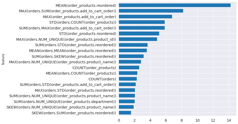
From the pipeline, we can see which features are most important for predictions.

feature_importance = best_pipeline.feature_importance
feature_importance = feature_importance.set_index('feature')['importance']
top_k = feature_importance.abs().sort_values().tail(20).index
feature_importance[top_k].plot.barh(figsize=(8, 8), fontsize=14, width=.7);

Next Steps

At this point, we have completed the machine learning application. We can revisit each step to explore and fine-tune with different parameters until the model is ready for deployment. For more information on how to work with the features produced by Featuretools, take a look at the Featuretools documentation. For more information on how to work with the models produced by EvalML, take a look at the EvalML documentation.